Machine learning can be characterised as the creation and application of algorithms that learn from data; the algorithms construct a trained model to reflect the input data. The intimation is that the algorithm in some way chooses a model that best fits the data. In reality the model has already been decided by the choice of the machine learning technique (e.g. if we employ linear regression, we are using a linear model). The ‘learning’ part can, therefore, be better characterised as choosing the number of parameters and their values – usually by trying to minimise some average error.
In contrast to statistics which places greater emphasis on inference – finding the model that best explains the data – machine learning emphasises a model’s predictive ability. With this in mind, we can form a list of problems that are suitable to a machine learning approach:
- Problems where there are no human experts, so data cannot be labelled or categorised;
- Problems where there are human experts, but it is very hard to program;
- Problems where there are human experts and it can be programmed, but where it is not cost effective to implement.
Problems that might not be well suited to a machine learning approach are those where causal inference is of primary interest, or where a physical model of a system can be produced based on insight beyond the raw data.
The first set of problems on the list, those where there are no human experts, is composed of unsupervised learning problems as there is no data with ground truth labels. These might include data exploration and hypothesis generation tasks, such as gene inhibitor problems; can a gene inhibitor be found amongst a set of potential candidates? The second set of problems in the list, where there are human experts capable of labelling data but it is hard to program, are composed of supervised learning tasks. An example of this would be character recognition; humans are very good at recognising handwritten characters, this makes it easy to produce a set of labelled training data. To program (let alone determine) all the rules required to recognise every type of handwriting, however, is incredibly complex. So it is easier to learn some general functions that have predictive power, based on labelled data. The final category, where there are human experts and you could in theory program all the rules, is composed of problems that change on a daily basis (such as the stock market), or where it is feasible to program but there are too many instances to program individually, e.g. a recommender system (like Amazon’s).
Stressing predictive ability over inference has associated issues. A model with a clear causal pathway should be able to cope with examples not seen in the raw data. In machine learning, however, it is possible to get a model that fits the training data perfectly but does not generalise to unseen examples. Poor generalisation is called over-fitting; where noise and errors in the training data have been misinterpreted as a useful signal. Below we consider an example of how to use machine learning to detect spam emails, and within this we show some methods that help prevent over fitting.
Spam emails are annoying; it’s best that they are filtered out. Humans are good at detecting which emails are spam, but the rules used by a human are complicated. Usually spam can be picked out from subtle – and sometimes not so subtle – signals such as strange grammar, and wild claims or requests. These signals are very hard to program as a set of rules, but a human can easily label emails as spam or not. Hence, identifying spam emails fits into the second category in our list of machine learning problems.
Detecting spam is a binary classification problem – emails either are or are not spam. There is labelled data (i.e. the emails in the training data are labelled as spam or not spam), so we can use supervised learning approaches. The challenge is to identify suitable features in the emails that can be mapped to the binary labels and thus be used to classify future emails as spam or not. The function used for the mapping must also be determined.
Features can be created by counting the occurrence of key words, this is called a bag-of-words approach. A key word list can be determined via expert judgement or by finding common words in the training set. To understand how the data is labelled, consider just two keywords “buy” and “$ $ $”. The count of occurrence of “buy” and “$ $ $” can then be labelled \(x_1\) and \(x_2\) respectively. A feature vector is \(x= (x_1,x_2 )\). In a real dataset there might be many thousands of features (key words). Since the training data is labelled, each feature vector is paired with a label \(y\). Spam emails are given a classification \(y = 1\), while non-spam emails have \(y = 0\). The training data can now be considered the set \( \{(x^{(i)},y^{(i)}) | i \in [1,m]\} \), where the superscript \(i\) denotes the training example, and \(m\) is the total number of training examples.
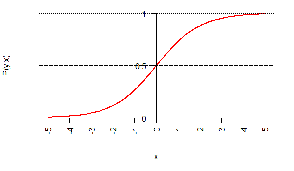
Binary classification is a problem suited to logistic regression. Logistic regression assumes that the conditional probability of having a spam email \((y = 1)\) given a set of features \((x)\) is equal to a sigmoid function with argument \(\Theta^T \cdot x\), i.e.
To train this classifier we use gradient descent, minimising the following objective function [1], which can be thought of as the classification error, to extract the values \(\Theta\). Determining the values of \(\Theta\) enables a decision boundary between data to be defined.
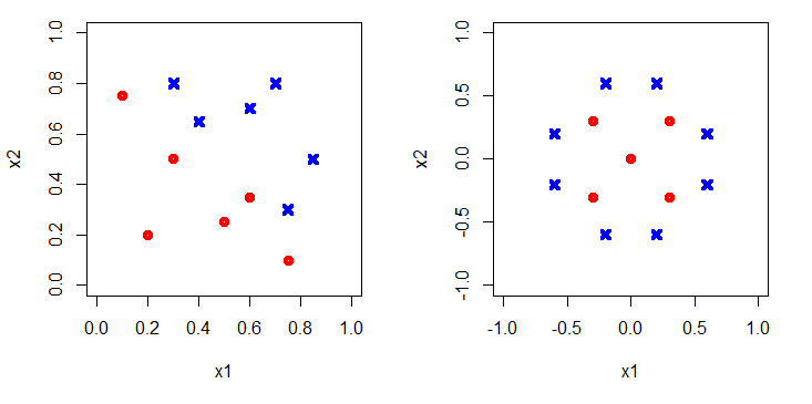
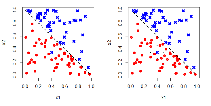
Figure 3 shows the decision boundaries added in. To capture the boundary on the left, the argument of the sigmoid function would have to be linear, e.g. \( \Theta_0 + \Theta_1 x_1 + \Theta_2 x_2 \), whereas to capture the non-linear circular boundary on the right a higher order polynomial would be required, e.g. \( \Theta_0 + \Theta_1 x_1 + \Theta_2 x_2 + \Theta_3 x_1^2 + \Theta_4 x_2^2 \). Clearly using a higher order polynomial will allow a better fit with the training data as there are more free parameters to choose. However, will it generalise well? Or will a too high order polynomial have been chosen meaning noise in the training data is fitted?
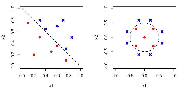
Figure 4 shows a different set of data, labelled in the same way. On the left a simple linear argument is used to fit the decision boundary. On the right a high order polynomial has been used. This successfully captures the blue dot that the linear boundary misclassifies.
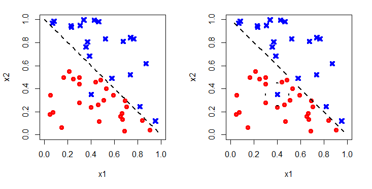
However, when more data are added, in Figure 5, it can be seen that the more complicated boundary gives many more misclassifications; the original training data was over-fitted.
So how do we get around this? How can we tell when the polynomial is of sufficiently high degree to characterise the data, but not too high that noise is fitted in the training data?
The answer is to split the training data into three. Data is randomly assigned to a training set, a cross-validation (CV) set and a test set. Typically the training set consists of 60%, the CV set 20% and the test set 20% of the data respectively. Next the model is trained using a number of different degrees of polynomial on the training data. For each model trained with a different degree polynomial, an error is determined on the CV set by evaluating the objective function. The polynomial giving the lowest error on the CV set generalises the best – it fits the training data and unseen CV data well. Hence this is chosen to form the final classifier. Finally, the generalisation error is determined from the test data. Neither the training nor the CV error are fair measures of generalisation error as information from these sets is used to pick the best hypothesis. Indeed the error on the test set is expected to be higher than on the CV set. A fair generalisation error is required to objectively compare between different types of model; we might for instance want to compare between a logistic regression model and a support vector machine.
There are many other techniques out there to make predictions from sets of data. All these techniques combined can be thought of as machine learning. If you would like to find out more about what mathematical approach is best suited to help you solve your business problems, please do get in contact.